Introduction
An analysis and synthesis of a 500 sample dataset was done in an effort to understand education in our different areas: gender, age, marital status and parental education. The descriptive statistics for various variables and the relationship between the variables are reported in this paper. Pearson’s correlation, regression analysis, ANOVA, and multivariate analysis of variance were some of the statistical tests conducted using this dataset. A discussion of the findings is given with reference to peer reviewed journals and finally a report – appropriate for a non-statistician audience -of the findings is provided.
Education and gender
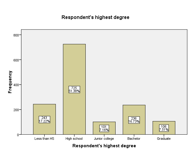
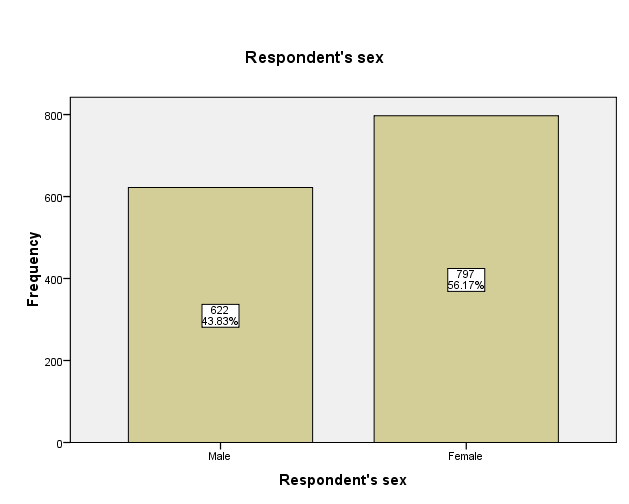
Among a total of 1419 participants who were involved in this study, there were 622 (43.8%) males and the rest 797 (56.2%) were females (Output 2). This information is also displayed graphically in Figure 3 where it is evident that there were more female participants than males. In addition, there were 8 missing data on highest degree in a total sample of 1419 participants. The highest number of respondents (725) had a high school degree (51%) while those who had less than a high school degree followed with 17.1% (243).
Individuals who had a bachelor degree were also substantially many, 236 (16.6%) while participants with a graduate degree were 106 (7.5%). Respondents who had a junior college degree were the least, 101 (7.1%). A graphical display of the respondents’ highest degree is also shown in form of a bar graph (Figure 1).
According to output 3 (Table 3), the mean highest year of school completed for male respondents was 13.54 with a standard deviation of 2.945. The 5% trimmed mean was 13.55 years and the median year of school completed was 13. The minimum highest year of school completed for males was 4 years whereas the maximum highest year of school completed was 20 years. This data is negatively skewed (-.013) and a kurtosis of.079 indicating that the data assumes normal distribution.
The mean highest year of school completed for female participants was 12.99 with a standard deviation of 2.834. The 5% trimmed mean was 13.03 and the median highest year of school completed was 12.00. The minimum highest year of school completed for females was 0 years whereas the maximum year is 20 years. This data has a negative skewness of -.249 and a kurtosis of 1.259 (output 3). It is conclusive that males have a higher level of education compared to females as far as highest year of school completed is concerned. In addition, it is possible to have females who have not completed one year in school but the least number of years completed by males is 4 years.
From output 4, the Pearson correlation coefficient between respondent’s gender and respondent’s highest degree (for a sample N = 1411) was significant, r = -.076, 2-tailed p =.004. It is important to note that the correlation is negative indicating that there is a significant negative relationship between gender and highest degree attained by respondents. Table 5 also shows that there was a significant relationship between gender of the respondent and the highest year of school completed for N = 1415, r = -.093, 2-tailed p <.05. Again this relationship is negative as indicated by the negative Pearson correlation coefficient. It is pertinent to note that there is a perfect correlation, r = 1 between each variable and itself.
The R2 value for gender against highest degree is (-.076)2 = 0.005776 which can be converted to 1%. This indicates that 1 percent variability in level of education (highest degree) was as a result of the individual’s gender. The R2 value for gender against highest year of school completed is -.0932 = 0.008649. When converted to a percentage, this becomes 1% indicating that 1 percent variability in level of education (highest year of school completed) was as a result of the participant’s gender. It is evident that although there was a significant relationship between gender and education, gender accounts for only 1% in level of education whereas the rest, 99%, is as a result of other variables.
Parental education and respondent’s education
The mean highest year school completed by mother is 11.56 with a standard deviation of 3.45 (N = 902) whereas for 902 participants, the mean highest year school completed by father is 11.37 with a standard deviation of 4.10 (output 6).
From the model summary in output 7, the R value is.362 indicating a somewhat strong correlation between parental education and the respondent’s education. The R2 value is.131 which is equivalent to 13.1 percent. This implies that parental education accounted 13.1 percent variation in respondent’s level of education. The remaining 86.9 percent was variation in respondent’s education due to other factors other than parental education.
The analysis of variance for this model is shown in Table 8. The average sum of squares for this model was 164.37 with 2 degrees of freedom. The F-ratio, 67.94 is significant at p =.001 (F (2 899) = 67.37, p =.001). The regression model therefore indicates that parental education significantly predicts the respondent’s education level. Output 9 is helpful in identifying the contributions of each parent’s education level on respondent’s education.
The Y intercept, b0 was.245 indicating that when x (parental education) is zero, the respondent’s level of education is.245. The two equations derived from Table 10 are Y =.086x +.245 for mother’s education and Y =.042x +.245 for father’s education. From the first equation, it is evident that when maternal education increases by a factor of 1, the respondent’s education increased by.086. Likewise, an increase in paternal education by a factor of 1 leads to an increase in respondent’s education by.042. It is therefore clear that maternal education has a higher contribution to respondent’s education compared to paternal education.
Maternal education has a significant contribution to respondent’s education as indicated by a significant t value, t = 6.24, p =.001. Paternal education also contributes to the respondents education significantly, t = 3.61, p =.001. The beta value for mother’s education is.25 whereas that of father’s education is.14 indicating that maternal education has a higher contribution to respondent’s education compared to paternal education.
Age and Education
Output 10 shows the mean age for 1409 respondents as 46.60 years with a standard deviation of 17.30. A Pearson correlation between respondent’s highest degree and the age of the respondent showed that there was a significant relationship, r = -.090, p =.001 for 1409 participants. The relationship was however negative indicating that as the age of the respondent increases, the highest degree achieved reduces. There exists a perfect relationship, r = 1, between every variable and itself. It is conclusive that age is a significant predictor of respondent’s education (highest degree).
Output 12 shows the model summary for this relationship and the r value is.090 showing that correlation between age of the respondent and respondent’s highest degree. The R Square value is.008, which is equivalent to 1% upon conversion to a percentage. This implies that although age is a predictor of respondent’s education, it causes a variability of 1% only with the rest 99% being variability due to other factors. The ANOVA for this model is shown in output 13 where the sum of squares was 15.84 whereas the mean square was 11.56 and 1 degree of freedom. The F-ratio was significant at p <.05 (F (1 1407) = 11.56, p =.001). This indicates that age is a significant predictor of the respondent’s education (highest degree).
From the regression coefficient in output 14, it is possible to indicate the exact effect of age on education. The regression equation in this case is Y = -.006x + 1.75 indicating that an increase in the respondent’s age by a factor of 1 leads to.006 decrease in respondent’s education (highest degree). When the respondent’s age is zero, the respondents education level is about -.006. The t value for this model is significant, t = -3.40, p =.001 indicating that age has a significant reduction in the respondent’s education. The beta value also shows that an increase in respondent’s age accounts for -.09 decrease in the respondent’s level of education.
When examining the contribution of age on respondent’s highest year of school completed, it is evident that the mean highest year of school completed was 13.23 with a standard deviation of 2.90 for 1413 respondents. For the same number of respondents, the mean age for respondents was 46.55 years (output 15). Table 16 shows the Pearson correlation coefficient for respondent’s age and highest year of school completed is significant, r = -.163, p =.001 (single- tailed).
The negative correlation indicates that as the age of the respondent increases, the highest year of school completed decreases. The R Square value is 0.027 which is equivalent to 2.7%. This shows that the respondent’s age has 2.7 % variability in the respondent’s highest year of school completed. The model summary in Table 17 shows that R =.163 which shows correlation coefficient of age and highest year of school completed, a weak relationship. The R Square value is.027 which is 2.7 percent variability of respondent’s highest year of school completed as a result of age.
Furthermore, the regression coefficient in output 18 shows that a change in the respondent’s age by a factor of 1 leads to a decrease in the respondent’s highest year of school completed by.027. When the respondent’s age is zero, the highest year of school completed is 14.50 hence the regression equation is Y = -.027x + 14.50. The beta value is -.163 indicating that a one unit variation in age causes a.163 decrease in highest year of school completed. Moreover, the t value is significant, t = -6.22, p =.001 indicating that respondent’s age causes a significant reduction in the highest year of school completed. While it is evident that the respondent’s education can be predicted by age, it is not possible to show the direction of causality as well as accounting for other variables other than age.
Marital status and education
On conducting a multivariate analysis on marital status and education, it was evident that there were 627 married participants, 139 widowed respondents, 228 divorced participants, 57 separated and 357 never married individuals (output 19). The multivariate tests showed a significant Wilks’ lambda.953, F = 8.62, df = 8 and p =.001. The Roy’s Largest Root as well as the Pillai’s Trace were also significant,.046, F = 16.28, df = 4.00 and p =.001 and.048, F = 8.55, df = 8.00 and p =.001 respectively. This is an indication that respondent’s education is significantly predicted by the respondent’s marital status.
The tests for between-subjects effects indicated that marital status significantly affects both the respondent’s highest degree as well as the highest year of school completed. The sum of squares for marital status influence on respondent’s highest degree was 57.51 while that of highest year of school completed was 515.89. The mean squares for respondent’s highest degree and highest year of school completed were 14.38 and 128.97 respectively and both had 4 degrees of freedom. The F values for highest degree and highest year of school completed were 10.78 and 16.03 respectively and both were significant, p =.001 for both (Output 21).
The R square for respondent’s highest degree is.030 indicating that marital status contributed 3% of variability in respondent’s highest degree. On the other hand, the R square value for highest year of school completed was.044 indicating that marital status caused 4.1% variability in respondent’s highest year of school completed. It can therefore be concluded that marital status has a higher contribution on respondent’s highest year of school completed than on respondent’s highest degree.
To identify which marital status actually caused a variation in respondent’s education, Tukey’s HSD post-hoc test was conducted. Tukey HSD test showed that there was a significant difference, mean difference of.68, p <.05 and 95% CI (.38 -.97), between married and widowed respondents in determining respondent’s highest degree. Tukey HSD test however showed that there was no significant difference between married and divorced, p =.77, mean difference of.10, 95% CI (-.14 -.35), and married and separated, p =.35, mean difference of.29, 95% CI (-.14 -.73) in determining respondent’s highest degree. Table 22 also shows that there was no significant difference between married and never married individuals in their contribution to respondent’s highest degree (mean difference =.02, p = 1.0, 95% CI (-.19 -.23)).
Tukey HSD indicate that there was a significant difference (p <.05) between widowed and divorced respondent’s in determining the respondent’s highest degree. This was also the case between widowed and never married individuals but there was no significant difference (p =.21) in respondent’s highest degree when comparing widowed and separated individuals. There was no significant difference in respondent’s highest degree when comparing divorced and separated as well as divorced and never married participants (p =.81 and p =.89 respectively).
However, a significant difference (p <.05) in respondent’s highest degree occurred between widowed and divorced individuals. There was no significant difference in respondent’s highest degree when comparing separated and all other forms of marital status (p >.05 for all cases) whereas there was a significant difference (p =.001) in highest degree when comparing never married and widowed participants.
Tukey HSD test also enabled the identification of the contribution of each marital status on the highest year of school completed. From Table 22, it is evident that there was a significant difference (p =.001) when comparing married individuals with widowed persons. However, there was no significant difference (p >.05) in highest year of school completed when comparing married and all the other forms of marital statuses.
When comparing windowed with married, never married and divorced individuals, there was a significant difference (p <.05) in highest year of school completed but no significant difference (p =.21) for widowed against separated individuals. There was no significant difference (p >.05) in highest year of school completed between all marital statuses and divorced individuals except for divorced against widowed persons (p =.001).
There was a significant difference (p =.04) in highest year of school completed between separated and never married individuals but no significant difference (p >.05) between separated and all other marital statuses. Finally, there was a significant difference in highest year of school completed between never married and widowed and never married and separated (p =.001 and p =.04 respectively) but no significant difference in highest year of school completed between never married and married never married and divorced (p <.05).
In summary, it is evident that married individuals tend to be more highly educated compared to single persons (whether divorced, separated, widowed or never married). However, these differences are not major as exemplified by the significant contributions of single-status of marriage for both highest degree as well as highest year of school completed.
Discussion-With Reference to Peer Reviewed Studies
The finding that there are differences in education as a factor of gender is an interesting one. In this analysis, it was evident that men have a slightly higher level of education than women. A study conducted by Allen et al. (2006) among Black men and Black women revealed a different pattern whereby it was identified that the enrollment of Black women in 4-year colleges was higher than enrollment for Black men. The increase in women than men in higher education was however noted to be a recent trend with enrolment rising from 54.5% in 1971 to 59.3% in 2004. Egun and Tibi (2010) also reported a gender gap in education particularly in Nigeria where there is an increasing enrolment of girls and a dwindling enrolment of boys.
These authors particularly cite an increase in girl enrolment in vocational subjects such as engineering. Although this difference is explained as resulting from sex-stereotyped occupations, it is a clear indication that there are emerging trends of education disparities among males and females. It is therefore conclusive that the findings of this study are not in tandem with recent findings on gender gap in education.
In general, it is observed that parental education has an influence on a child’s education in the form of intergenerational transmission of capital. Behrman and Rosenzweig (2002) examined the effects of educating women on the next generation and stated the existence of a relationship. In particular, these authors identified that mothers who had more schooling tended to have children who have a higher schooling.
This therefore confirms that there is a relationship between parental education and the education of the child whereby the strongest effect on child education is as a result of mother’s education. It is important to note that Behrman and Rosenzweig (2002) used homozygous twins as a way of controlling for any genetic factors as well as marital sorting. While there was a significant increase in child education due to increase in maternal schooling, there was also a significant increase in child education due to increase in paternal education. It is therefore conclusive that the findings from the current data on parental education and child education are in tandem with pervious studies.
However, the current findings do not provide for the possible causes in the differences in effect of parental education on child’s education. Similar findings have also been reported by Curie and Moretti (2003) who identified that maternal education impacts heavily on child education in the process of intergenerational transmission. These authors argue that other than health benefits accrued due to higher maternal education, improved child education also comes along as a spill-over effect.
There exists a relationship between age and education. Owen (2003) explained this relationship by citing that age positively correlated with Grade Point Average (GPA). Owen explains that GPA helps in measuring academic success and therefore the higher the GPA, the higher the academic success. In the study among 158 adult students (18 years and above), this author identified that as age increased, there was a slight increase in GPA. While this finding seems to contradict the findings from the above analysis, it is notable that this study used GPA measure as opposed to highest degree in this paper. Owen (2003) however indicates that as age increased, there was a reluctance to enroll back into college thus agreeing with the findings that as age increases, education level decreases.
There is a noted influence of marital status on education whereby it has been recorded that most educated individuals tend not to be married. Bruderl and Diekmann (1997) indicate that as the level of education increases, the likelihood to delay marriage increases. As such, it is expected that most singles have a higher level of education than married individuals. Our analysis does not differ with these findings since it is already stated that the mean age for this population is 46.60 (Table 15). With a mean age of 46.6 years, it is expected that most individuals are married and this is practically true since the married individuals constituted the majority (627).
It is therefore negated that single adults have a higher education attainment compared to married adults. Stevenson (2010) points out that there has been an increase in individuals studying at an older age which is also related to later marriage. Taking note of the older person’s having a higher level of education, it is apparent that findings from this study conflict with findings in some studies.
According to a recent publication by Isen and Stevenson (2010), there is a changing trend in marriage and education whereby there has been an increasing trend of more college level women marrying and remarrying. Also notable is that the trend has changed for men but at a very slow rate. The findings from this paper that married individuals tend to have a higher education are therefore in line with recent findings as observed in Isen’s and Stevenson’s (2010) study.
A Report for a Non-Statistician Academic Conference on Adult Education
In a study conducted among 1411 adults, it was identified that a majority of adults have acquired high school degree (51.1%) with a substantially high proportion (17.1%) having less than a high school degree. While almost an eighth (16.6%) has a bachelor degree, the percentage of graduates is even lower (7.5%). The lowest numbers of adults have a junior college degree (7.1%; Table 1).
While examining education based on gender, it is clear that males have a higher level of education compared to women. Most men have completed 13 years of schooling as compared to 12 years among women. In addition, the least number of years of school completed among men is 4 years whereas there are females who have not completed even a single year in school (minimum completed year of school is 1; Table 3).
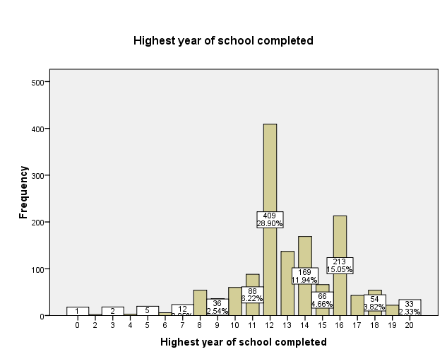
It is however notable that both males and females have the opportunity of completing the highest number of years in school (20 years). Looking at males and females, the highest number of years of school completed is 12 (Figure 2) implying that most males and females have at least a high school degree. It is therefore important to note that there is a gender gap in education with more males attaining higher levels of education as compared to females. However, the difference in education due to gender is very minor and therefore there must be other factors that affect the education gap between males and females.
The level of education that parents have attained reflects the level of education of their children. To be precise, parents who have a higher level of education have an influence on their children’s education such that their children also tend to have a higher level of education. It is important to note that both parents tend to have the same education more so in terms of highest years of education completed (Table 6).
However as much as both parents’ education influences the child’s education level positively, the influence of mother’s education is more powerful. The higher the level of education a mother has, the higher the level of education achieved by the child. It can therefore be concluded that mother’s education has a greater positive intergenerational transfer compared to father’s education.
Age is a determinant of an individual’s education level. In specific, the relationship between age and education is that an increase in age tends to be associated with a lower level of education achievement. It is therefore expected that adults with an older age have completed a fewer years in school compared to adults with a younger age. It is however notable that age is only a minor contributor on a person’s education (Table 12) and therefore other factors play a significant role in determining an individual’s educational achievement. It is also important to note that as an individual’s age increases, the highest year of school tends to decrease by a factor of 2.7% (Table 17). In the same manner, the highest degree attained also decreases by a small factor (1%; Table 12).
Level of education among adults is significantly dependent on marital status. In deed, martial status influences an individual’s highest degree by about 3% whereas the individual’s highest year of school completed is influenced by 4.1% (Table 21). Upon examining the significance of the various marital statuses in influencing education, it is clear that married individuals tend to have higher level degrees and more years of school completed than their single counterparts.
Among the various groups of singles, widowed individuals tend to have better educational achievements than the separated, divorced or never married persons. Separated and never married individuals instead have an overall lower educational achievement. In summary, adult education is determined by various factors which bring various disparities. Gender and marital status gaps are evident in adult education whereas age and parental education greatly influence educational achievements among individuals.
References
Allen, W. R., Jayakumar, U. M., Griffin, K. A. Kom, W. and Hurtado, S. (2006). “Black undergraduates from Bakke to Grutter: freshmen status, trends and prospects, 1971-2004.” The Journal of Pan African Studies, 1(3): 106-109.
Behrman, J. R. and Rosenzweig, M. R. (2002). Does increasing women’s schooling raise the schooling of the next generation? The American Economic Review, 92(1): 323-334.
Bruderl, J. and Diekmann, A. (1997). Education and marriage: A comparative study. Journal of Marriage and the Family 54: 302-315.
Currie, J. and Moretti, E. (2003). Mother’s education and the intergenerational transmission of human capital: Evidence from college openings. Quarterly Journal of Economics, VCXVIII(4): 1495-1532.
Egun, A. C. and Tibi, E. U. (2010). The gender gap in vocational education: Increasing girls access in the 21st century in the Midwestern states of Nigeria. International Journal of Vocational and Technical Education, 2(2): 18-21.
Isen, A. and Stevenson, B. (2010). Women’s education and family behavior: Trends in marriage, divorce and fertility. CESifo Working Paper Series 2940, CESifo Group Munich.
Owen, R. T. (2003). Retention implications of a relationship between age and GPA. College Student Journal, 37(22): 181-190.
Stevenson, B. (2010). Who’s getting married? Education and marriage today and in the past: A Briefing Paper Prepared for the Council on Contemporary Families. Web.
Appendix
Table 1: A Frequency Table for Respondent’s Highest Degree.
Table 2: A Frequency Table for Respondent’s Gender.
Table 3: Descriptive Statistics for Male and Female Highest Year of School Completed.
Table 4: Pearson Correlation between Respondent’s Gender and Respondent’s Highest Degree.
Table 5: Pearson Correlation between Respondent’s Gender and Highest Year of School Completed.
Table 6: Descriptive Statistics for Highest Year School Completed (Mother and Father).
Table 7: Model Summary for Highest Year School Completed.
Table 8: ANOVA for Highest Year of School Completed by Father and Mother.
Table 9: Regression Coefficients between Highest Year of School Completed by Mother and Father.
Table 10: Descriptive Statistics for Age of the Respondents and Highest Degree.
Table 11: Pearson Correlation between Respondent’s Age and Respondent’s Highest Degree.
Table 12: Model for Age as a Predictor Variable.
Table 13: ANOVA for Respondent’s Age and Respondent’s Highest Degree.
Table 14: Regression Coefficients for Respondent’s Age and Respondent’s Highest Degree.
Table 15: Descriptive Statistics for Age of the Respondent and Highest Year of School Completed.
Table 16: Pearson Correlation between Age and Highest Year of School Completed.
Table 17: Model Summary for Age of the Respondents.
Table 18: Regression Coefficients for Age of the Respondent against Highest Year of School Completed.
Table 19: Between-Subject Factors for Marital Status.
Table 20: Multivariate Tests for Marital Status.
Table 21: Tests of Between-Subjects Effects for Respondent’s Education.
Table 22: Post-hoc Test (Tukey HSD Test) for Marital Status and Education.